How to Make Flow Field Line Art with Flow Lines

What a vector field is

Flow field art starts with a rule that gives every point on the page a direction. Flow Lines writes that rule as two formulas: X Formula gives the horizontal push at a point and Y Formula the vertical push, both as functions of the point’s coordinates x and y. Together they form a vector field F(x, y).

A streamline is the path a particle would follow if it always moved in the field’s direction. The tool traces streamlines from many starting points and stops each one when it comes too close to another, so the lines stay evenly spaced instead of bunching up. The result is a set of open polylines, which is exactly what a pen plotter wants: no fills, no overlapping strokes, one continuous line per path.

The page covers the square from −5 to 5 in both directions, mapped onto 800 × 800 SVG units. Formulas are evaluated in those maths coordinates, so sin(x) completes about one and a half waves across the page.

Trace your first field

1. Open Flow Lines. The default field is cos((cos(y) - x * y)) for X and x for Y.
2. Edit either formula and the streamlines retrace as you type. Try 1 for X and 0 for Y to see plain horizontal lines, then bring the original formulas back with the reset buttons.
3. Press 🎲 Randomize to grow a brand-new pair of formulas from an expression grammar. The arrows beside it move back and forward through your history.
4. Click Download SVG. Every streamline becomes one <polyline>, and the settings are written into the page URL so Copy Link reproduces the design.

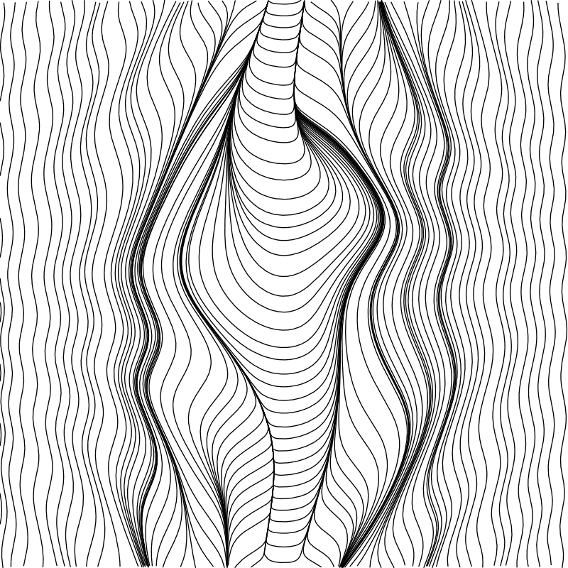
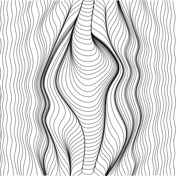
Open this design in Flow Lines · settings: defaults

Three worked examples

Cells: sine and cosine

sin(y) for X and cos(x) for Y gives a field that circulates around a grid of centres. Every streamline curls into a closed cell.

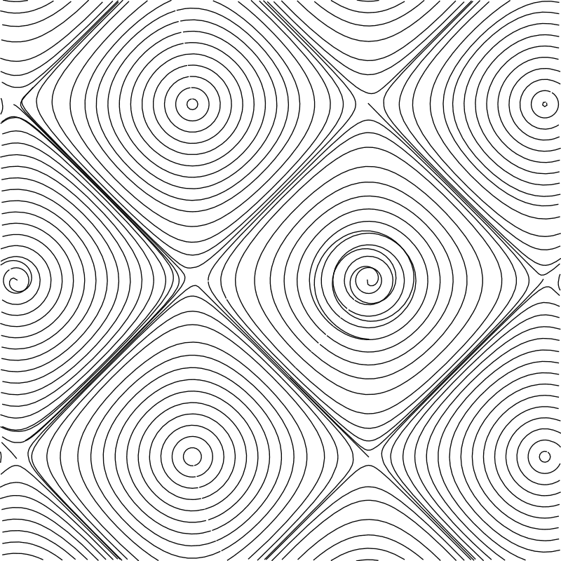
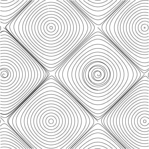
Open this design in Flow Lines · settings: X sin(y) · Y cos(x)

Saddle: mixing a polynomial with a wave

y-x*x/4 for X and sin(x) for Y combines a parabola with a wave. Streamlines flow around two eyes near the top and pass through a saddle in the middle, giving the drawing an obvious focal point.

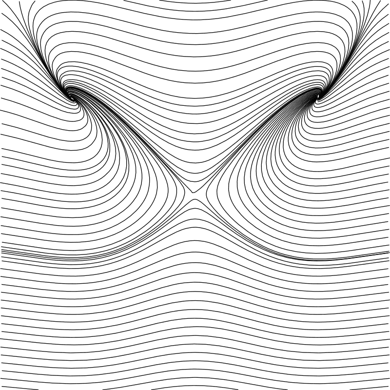
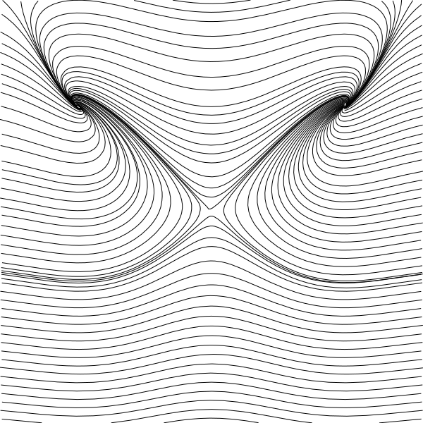
Open this design in Flow Lines · settings: X y-x*x/4 · Y sin(x)

Your own field

Good fields mix a slow term with a fast one. Start from x and y, add a sin or cos of the other coordinate, and scale the argument (sin(2*y) doubles the number of waves). Fields that only rotate, such as y and -x, draw perfect circles; fields that only push, such as 1 and 0.5, draw parallel lines. Interesting drawings usually sit between the two.

Eight favourite streamline plots

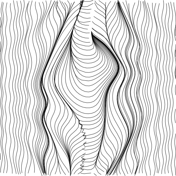
These are Flow Lines drawings Maks kept from the tool’s first years, exported at 600 × 600 units and plotted since. That early version did not write its formulas into the file, so unlike the Rad Lines favourites they cannot be reopened with a link; they are here as finished, plottable SVGs to download, and as a picture of what the tool can do once you move past the defaults. The current tool records every setting, including the seed, in the SVG’s <title> element, so files you export today can always be reproduced.

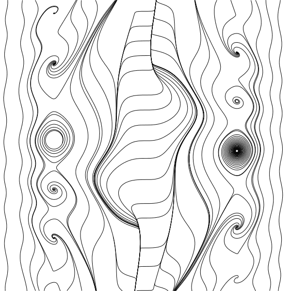
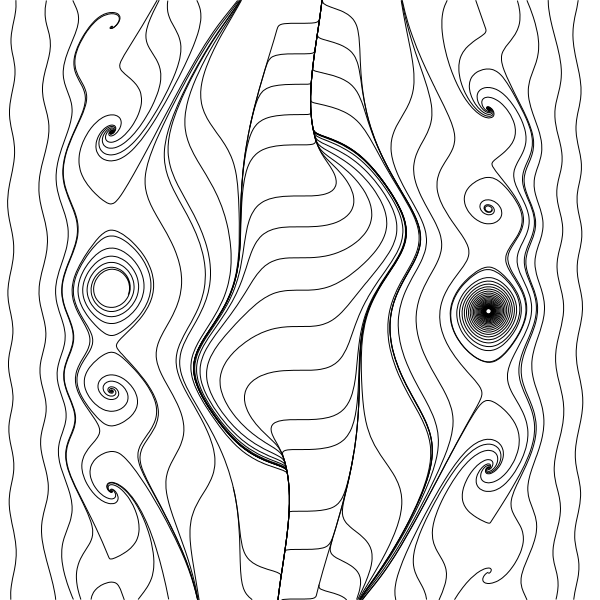
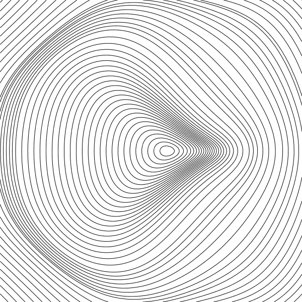
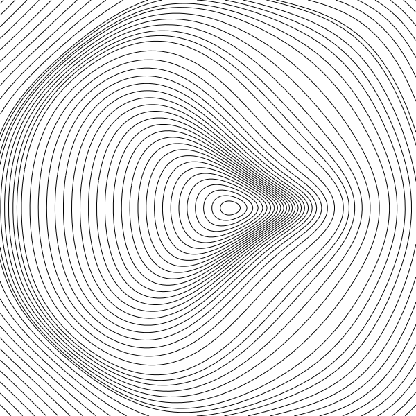
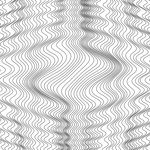
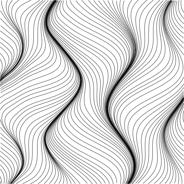
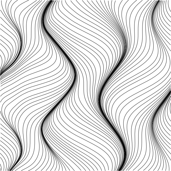
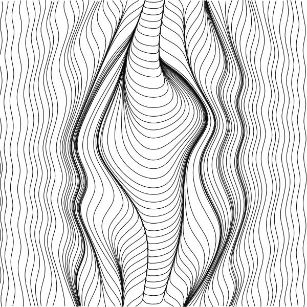
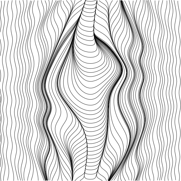
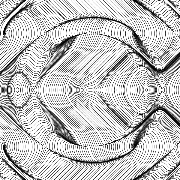
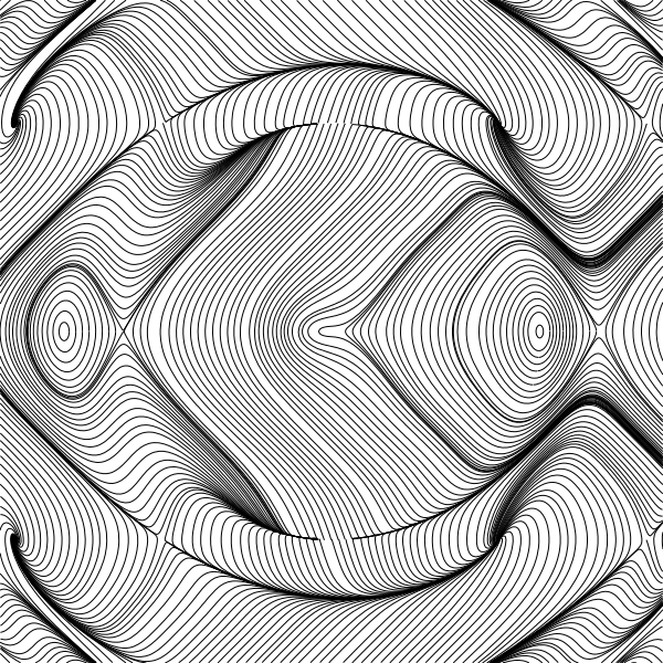
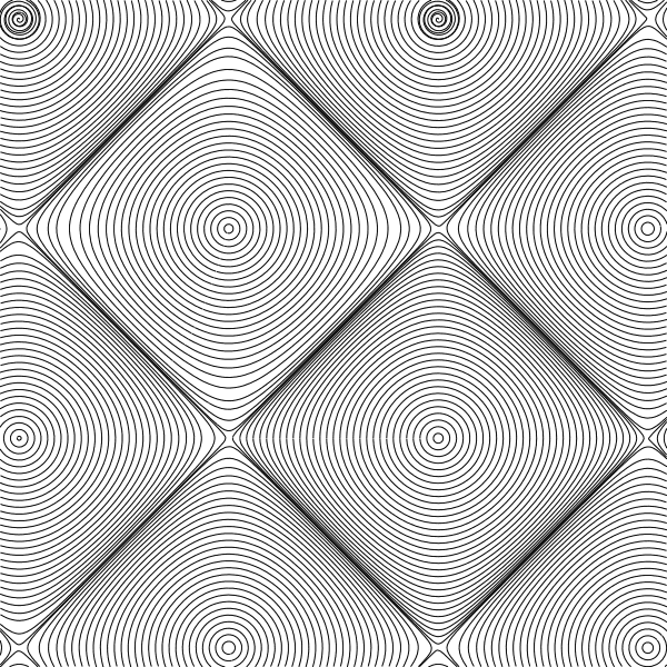
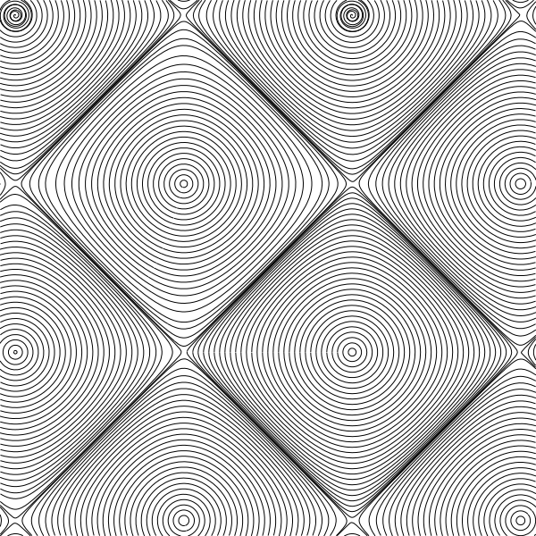
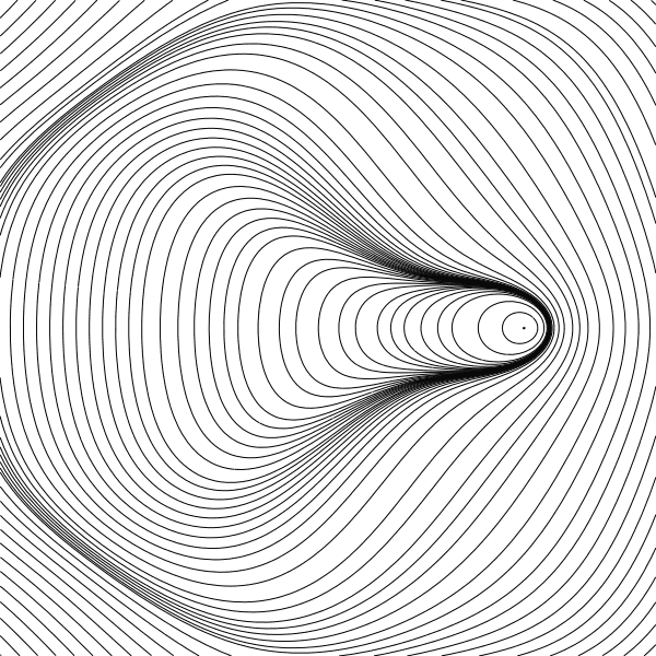
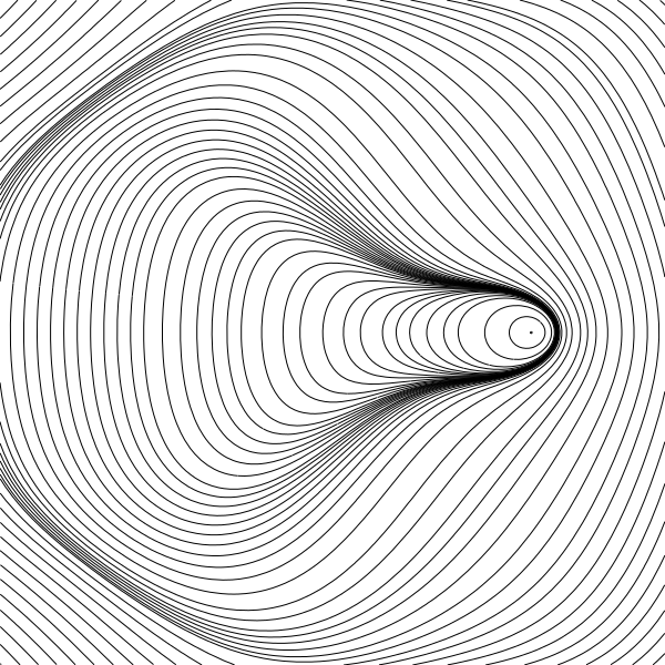
A few things to take from them. Vortices and eyes come from fields with a rotational term, such as y in the X formula paired with -x in the Y formula, or a sin of the other coordinate. Repeating cell patterns like the diamonds come from products such as sin(x)*cos(y). Line count is the plot-time budget: the nested rings have almost seven times as many pen strokes as the vortices. Open a favourite in Plot Preview to see it at your paper size with your pen before committing to it.

Density, detail and file size

Four numeric settings decide how many lines are drawn and how many points each one carries. The comparison below keeps the default field and changes one value at a time.

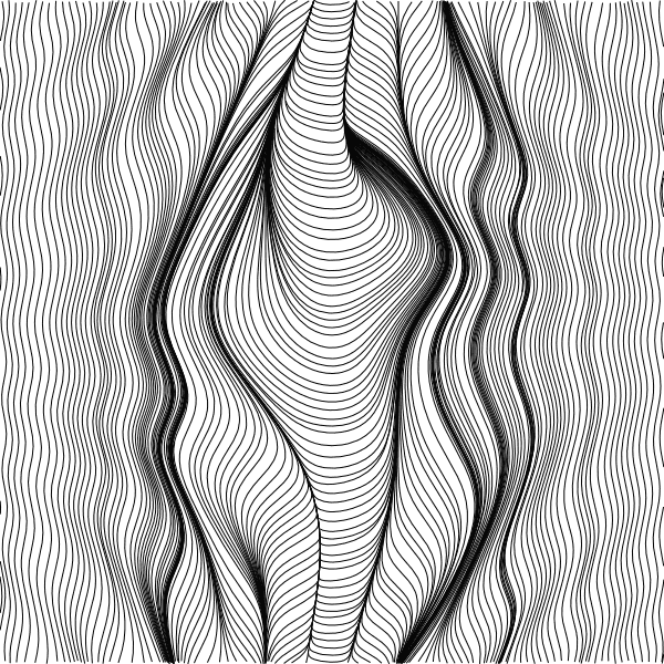
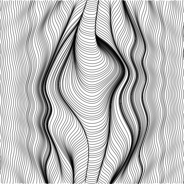
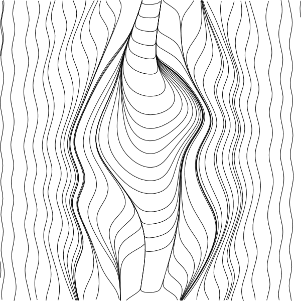
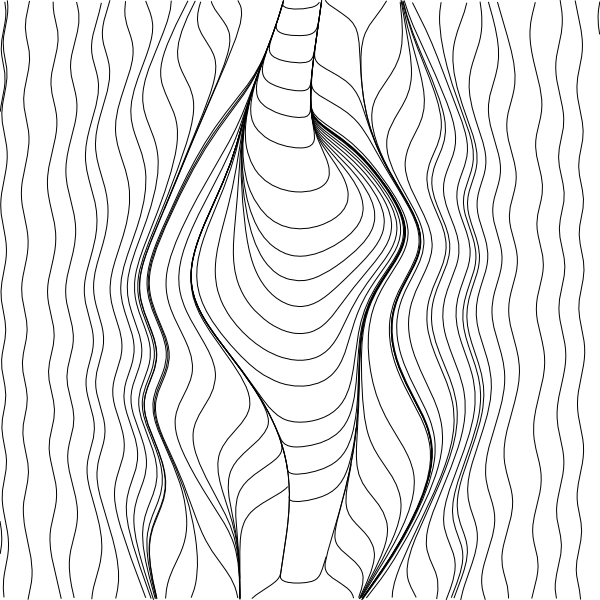
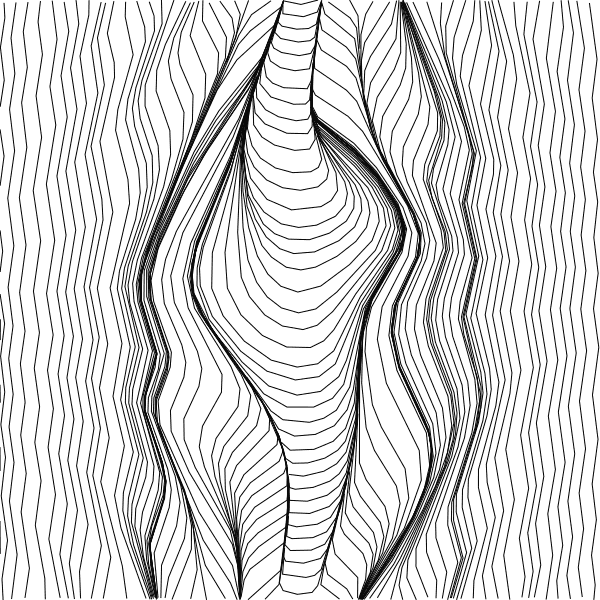
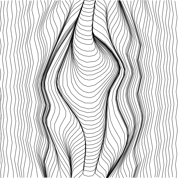
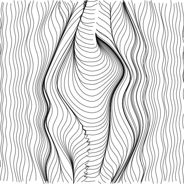
• Separation Distance is the gap between the starting points of neighbouring streamlines. Halving it from 0.2 to 0.1 roughly doubles the line count and the plotting time.
• Stop Distance (dTest) is how close a streamline may come to an existing one before it stops. Keep it well below the separation distance; raising it shortens lines and opens gaps.
• Time Step is the integration step. Smaller steps follow tight curves more faithfully but add points; 0.2 is visibly coarser around the vortex.
• Simplification removes points that do not change the shape by more than the tolerance in page pixels. A value of 2 cut the default design from about 6,300 points to 1,900 with no visible change at plot size.

The default drawing downloads at about 88 KB. For a plotter, point count matters less than line count: each streamline costs a pen lift, so Separation Distance is the setting that decides plot time.

Stroke and background

Stroke Width and Stroke Color only affect the appearance of the file on screen. The plotter follows the centreline of each polyline with whatever pen is loaded; a 0.3 mm technical pen and a 1 mm brush pen will draw the same paths with very different results. Use the stroke width to judge spacing, then verify at size in Plot Preview.

Background adds a filled rectangle behind the lines. Most plotting software will try to draw or fill it, so leave it off when exporting for a machine and use it only for screen previews. A white or dark background is useful when picking a stroke colour for a coloured paper.

Prepare the SVG for plotting

• Open the download in SVG Optimizer. Sort for Plotting reorders the streamlines to reduce pen-up travel between them, and Merge Lines joins lines whose ends touch; the before/after slider confirms the drawing is unchanged.
• Use SVG Effects to hatch areas, warp the field, or layer a second copy in a different colour for a two-pen plot.
• Check the physical size in your plotting software. The file’s viewBox is 800 × 800 units; the page size in millimetres is set when you import it.

Common problems:

• Nothing is drawn: the formulas produced NaN or infinity, for instance 1/x at x = 0. Add a small offset such as 1/(x+0.01).
• Only a few long lines: the field is nearly uniform. Add a term that varies with the other coordinate.
• Lines break into short dashes: Stop Distance is too close to Separation Distance. Lower it.
• The file is very large: raise Simplification before lowering Separation Distance.

Figures on this page are browser exports rasterised for the web; no physical plot of them is claimed. For radial designs, see the Rad Lines guide.